Combining Forecasts (Part 2)
We’ll continue to explore ways to combining multiple forecasts.
10.1 Weighting Experts
Last time, we discussed the weighted mean as a candidate approach to combine point estimates. This approach requires figuring out weights for each expert. But how do we come up with these weights?
As a motivating example, let’s consider the forecasting question from a past homework:
On February 1st at 2pm EST, the U.S. Federal Reserve (the Fed) is planning to announce interest rates. Note that the federal interest rate is a range (e.g. 5% − 5.25%). What will be the upper value of this range?
When I was come with a forecast for this question, I consulted several sources, summarized below.
“We are changing our call for the February FOMC meeting from a 50 [basis point] hike to a 25bp hike, although we think markets should continue to place some probability on a larger-sized hike.” (source, Jan 18)1
“Pricing Wednesday morning pointed to a 94.3% probability of a 0.25 percentage point hike at the central bank’s two-day meeting that concludes Feb. 1, according to CME Group data.” (source, Jan 18)2
“Markets expect the Fed to raise rates again on February 1, 2023, probably by 0.25 percentage points…. However, there’s a reasonable chance the Fed opts for a larger 0.5 percentage point hike.” (source, Jan 2)3
Before continuing to read, think through how you would weight these sources.

One way to combine up with weights for experts is to look at past track record. We could even improve this by tracking what type of questions they are good at.
We can formalize this mathematically by conceptualizing each forecast is as a noisy estimate of the truth, where different forecasts have different noise levels. Given this interpretation, to assign each forecast a weight, what we really want to do is to convert noise levels into weights.
10.1.1 Converting Noise Levels into Weights
We’ll describe a mathematical approach to convert noise levels into weights. Although this approach is hard to literally use in practice, it has good conceptual motivation. In fact, this approach is “optimal” under some assumptions (though these assumptions may not always be true). More specifically, if estimates are unbiased and independent, and estimate i has standard deviation \(\sigma_i\), then we’ll show that the weights should be proportional to \(1/\sigma_i^2\).
Assume there is some “true” quantity we are trying to estimate (e.g. how the forecast will actually resolve), which we denote \(\mu\). We have several noisy “signals” about this quantity, which we’ll denote \(X_1, \ldots, X_n\). Think of these as the estimates we get by consulting different reference classes. Model each \(X_i\) as a random variable, and assume that it has mean \(\mu\) (it is in expectation an accurate signal) and standard deviation \(\sigma_i\) (it has some error). In other words: \[ \mathbb{E}[X_i] = \mu, \text{Var}[X_i] = \sigma_i^2\]
Our goal is to combine these signals together in the best way possible. Suppose we decide to combine them by taking some weighted sum, \(\sum_i w_i X_i\). Then, we need to have \(\sum w_i = 1\) (so that the weighted sum also has expectation \(\mu\)). The best weights will be the ones that minimize the variance of the sum.
First, assume the \(X_i\) are independent (i.e. each reference class has independent errors relative to the true estimate). We can compute the variance as
\[\text{Var}[\sum_{i=1}^n w_i X_i] = \sum_{i=1}^n w_i^2 \text{Var}[X_i] = \sum_{i=1}^n w_i^2 \sigma_i^2.\]
Our goal is to pick weights to minimize this variance subject to the constraint that \(\sum_{i=1}^n w_i = 1\). We can show that4
\[w_i \propto \frac{1}{\sigma_i^2}.\]
Interpretation: A variance typically corresponds roughly to the \(70\%\) confidence interval for a random variable. So if we have confidence intervals obtained from several difference “signals” of the same underlying ground truth, and we think that each signal makes independent errors, the weight for each signal should be proportional to the inverse square of its confidence interval. In practice, I think this is a bit too aggressive, mainly because most errors are not independent in practice. So I tend to take weights that are closer to \(\frac{1}{\sigma_i}\), i.e. the inverse (not inverse square) of the confidence interval width. But I’m not confident this is correct–under some assumptions, dependent errors imply that we should place even more weight on smaller values of \(\sigma_i\).
Generalization to dependent errors: If the errors are dependent, we should intuitively downweight estimates that are more correlated with others. We can formalize this intuition using a bit of linear algebra, although the resulting formula isn’t necessarily that illuminating. Suppose that we have the same setup as before with \(\mathbb{E}[X_i] = \mu\). Since the errors are now dependent, we need to consider the covariance between every pair of \(X_i\), \(X_j\), so let \(S_{ij} = \text{Cov}(X_i, X_j)\), in which case \(S_ii = \sigma_i^2\) is the variance of \(X_i\). Then, the formula for the variance of \(\sum_i w_iX_i\) is
\[w^{\top}Sw = \sum_{i,j=1}^n w_iw_j S_{ij}\]
Taking derivatives and setting to zero, we find that we should choose weights \(w\) proportional to \(S^{-1}\mathbf{1}\), which is the inverse-covariance matrix multiplied by the all-1s vector. Somewhat oddly, this can lead to negative weights in some cases.
10.2 Working in Teams: The Delphi Method
Beyond assigning weights to forecasts, another way to take advantage of multiple perspectives is to allow the forecasters to work together and share their reasoning with each other.
The Delphi method is where forecasters individually come up with predictions and reasoning and then provide predictions and reasoning to the group. Individuals update based on group forecast, potentially over multiple arounds. At the end, the group creates a forecast by taking an average of all of the final individual forecasts.
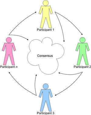
Intuitively, this approach benefits not only from averaging, but also discussion—you can improve your estimates of intermediate quantities or improve what your reference classes you consider by discussing with others.
There are several variants to the Delphi method. For example, predictions and reasoning can be provided anonymously. Or, only reasoning is shared with the group, not numerical predictions.
10.3 Combining Confidence Intervals
So far, we’ve focused on combining point estimates. But what if we want to combine confidence intervals? That is, if each forecaster gives us a confidence interval, how should we come up a confidence interval that combines all of their estimates?
The simplest approach is to take the mean (or the trimmed mean) of the upper and lower endpoints. However, this can be an underestimate (e.g., if the intervals are disjoint) or not end up being dominated by some large intervals (e.g. if some intervals are over different orders of magnitude than other intervals).
Here is a more sophisticated approach to combine intervals, that uses mixtures. Suppose we have confidence intervals \([a_1, b_1], \ldots, [a_n, b_n]\), and we want to combine these together. Conceptually, we can think of each confidence interval \([a_i, b_i]\) as a probability distribution \(p_i\) such that \(a_i\) and \(b_i\) are upper and lower percentiles of \(p_i\). We then want to make a new forecast based on averaging these distributions, to obtain \[\bar{p} = \frac{p_1 + \ldots + p_n}{n},\] where the sum denotes the mixture of distributions. (As an example, if all of the distributions \(p_i\) are equal to some distribution \(p\), then the average distribution \(\bar{p}\) is also equal to \(p\).)
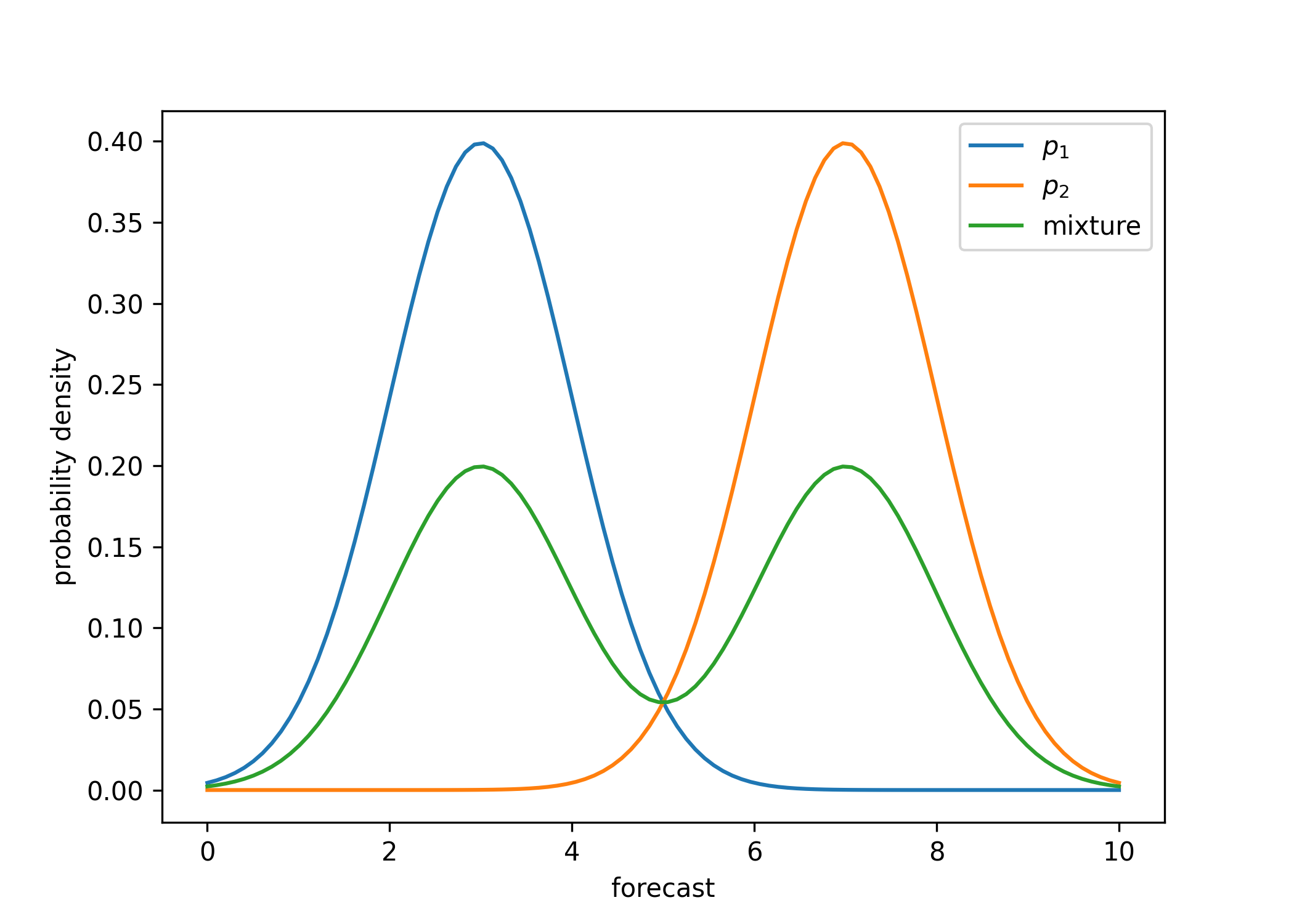
Sampling from \(\bar{p}\) is not the same as taking the average sample from the \(n\) distributions. Instead, a correct way to get a sample from \(\bar{p}\) is to sample uniformly from \(i \sim \left\{1, 2, \ldots, n\right\}\) and then take a sample from \(p_i\).
We would like the upper and lower confidence intervals of this new distribution \(\bar{p}\). How can we get that?
10.3.1 Basic Formulation of Mixture-Based Confidence Interval
First, let’s use the heuristic that being within one standard deviation corresponds to the 70% confidence interval of \(p_i\). So \(p_i\) is a distribution with variance \(\sigma_i^2\) roughly proportional to \((b_i-a_i)^2\). What, then, is the variance of \(\bar{p}\)?
It turns out the variance \(\text{Var}(\bar{p})\) depends on the means of each \(p_i\) as well, so suppose that each \(p_i\) has mean \(\mu_i\). (One way to approximate \(\mu_i\) is as \((a_i + b_i)/2\), although we might want to use a different value if we think the distribution is left- or right-skewed.) Observe that \(\bar{p}\) has mean \[\bar{\mu} = \frac{\mu_1 + \ldots + \mu_n}{n}.\] The variance is a bit trickier to compute, but can be calculated as the average of the variances plus the variance in means5: \[\text{Var}(\bar{p}) = \frac{\sigma_1^2 + ...+ \sigma_n^2}{n} + \frac{(\mu_1 - \bar{\mu})^2 + \cdots + (\mu_n - \bar{\mu})^2}{n}.\]
Turning this back into confidence intervals, we want a confidence interval centered at \(\bar{\mu}\) with width given by \(\bar{\sigma}\), That is: the combined confidence interval is
\[[\bar{\mu} - \bar{\sigma}, \bar{\mu} + \bar{\sigma}]\]
where
\[\bar{\sigma} = \sqrt{\frac{\sigma_1^2 + ...+ \sigma_n^2}{n} + \frac{(\mu_1 - \bar{\mu})^2 + \cdots + (\mu_n - \bar{\mu})^2}{n}}.\]
To unpack this formula, let’s consider several examples. The simplest case is where all of the confidence intervals are equal to \([a, b]\): in this case, the combined confidence interval would also be equal to \([a, b]\). As another example, if all of the confidence intervals have the same mean but different widths, then the second term is equal to \(0\): this means the combined confidence interval width is equal to the quadratic mean of the widths of the original confidence intervals. If the means are different, then the second term serves as a penalty that increases the combined confidence interval width.
10.3.2 Adjustments to Mixture-Based Confidence Interval
The confidence interval above doesn’t account for two additional things we care about:
- The width should depend on the actual interval probability we are using, e.g. 70% vs 80% vs 90%. The derivation above is mostly about the 70% interval due to the “70% = standard deviation” heuristic.
- We want to account for skewness—if the original intervals are left- or right-skewed, we want our final one to be as well.
Here is a heuristic formula that has both of these properties as well as approximately the correct width: Let \(\mu_0\) be the overall mean estimate (or the median of the interval centers, or any other good guess of the center of the distribution). Choose the following confidence interval:
\[\left[\mu_0 - \sqrt{\frac{\sum_{i=1}^n (\mu_0 - a_i)^2}{n}}, \mu_0 + \sqrt{\frac{\sum_{i=1}^n (b_i - \mu_0)^2}{n}}\right]\]
Why is this a reasonable estimate? This confidence interval is centered at \(\mu_0\) (the mean) and has lower width \(\sqrt{\frac{\sum_{i=1}^n (\mu_0 - a_i)^2}{n}}\) and upper width \(\sqrt{\frac{\sum_{i=1}^n (b_i - \mu_0)^2}{n}}\). If all of the confidence intervals are equal to \([a,b]\) and \(\mu_0\) is the mean of the interval centers, then the proposed confidence interval would also be \([a,b]\). More generally, if \(\mu_0\) is the mean of all of the interval centers, then we can interpret \(\frac{1}{2} \left(\frac{\sum_{i=1}^n (\mu_0 - a_i)^2}{n} + \frac{\sum_{i=1}^n (b_i - \mu_0)^2}{n}\right)\) as the variance of the distribution given by sampling the interval endpoints \(a_i\) and \(b_i\) uniformly at random. The proposed confidence intervals essentially uses this as the width, but treats the lower and upper bounds separately.
10.4 Summary
Let’s end with a summary of what we’ve learned about combining forecasts from the past 2 lectures.
Averaging multiple approaches or experts often improves forecasts.
Assess track record and accuracy of sources to determine weights.
Consider working in teams and generating independent numbers.
Combining confidence intervals: several ideas, but there is no silver bullet (yet).
Shared by an economist at Citigroup, the 3rd largest banking institution in the US↩︎
Based on CME Group data. The CME Group is the world’s largest financial derivatives exchange. The CME FedWatch Tool uses futures pricing data (the 30-Day Fed Funds futures pricing data) to analyze the probabilities of changes to the Fed rate.↩︎
From Simon Moore who is a writer at Forbes. He provides an outsourced Chief Investment Officer service to institutional investors. He has previously served as Chief Investment Officer at Moola and FutureAdvisor, both are consumer investment startups that were subsequently acquired by S&P 500 firms. He has published two books and is a CFA Charterholder and educated at Oxford and Northwestern.↩︎
Recall that our goal is to minimize \(\sum_{i=1}^n w_i^2 \sigma_i^2\) subject to the constraint \(\sum_{i=1}^n w_i = 1\). To do this, we use Lagrange multipliers. The Lagrangian is: \[L(w_1, \ldots, w_n, \lambda) = \sum_{i=1}^n w_i^2 \sigma_i^2 - \lambda \left(\sum_{i=1}^n w_i - 1\right).\] The partial derivative of \(L\) with respect to \(w_i\) is: \[\frac{\partial L}{\partial w_i} = 2 \sigma_i^2 w_1 - \lambda.\] Setting this equal to \(0\), we obtain: \[w_i = \frac{\lambda}{2 \cdot \sigma_i^2}\] which proves that the weights are proportional to \(1/\sigma_i^2\).↩︎
The variance \(\text{Var}(\bar{p})\) is equal to \(\frac{1}{n} \sum_{i=1}^n \mathbb{E}[p_i^2] - (\bar{\mu})^2\), which is equal to \(\frac{1}{n} \sum_{i=1}^n (\sigma_i^2 + \mu_i^2) - (\bar{\mu})^2\), which is equal to \(\frac{\sigma_1^2 + ...+ \sigma_n^2}{n} + \frac{1}{n} \sum_{i=1}^n \mu_i^2 - (\bar{\mu})^2\). The second term is equal to the variance of the distribution given by uniformly choosing \(\mu_1, \ldots, \mu_n\) at random and can be equivalently written as \(\frac{1}{n} \sum_{i=1}^n (\mu_i - \bar{\mu})^2\).↩︎