Common Probability Distributions
When we output a forecast, we’re either explicitly or implicitly outputting a probability distribution.
For example, if we forecast the AQI in Berkeley tomorrow to be “around” 30, plus or minus 10, we implicitly mean some distribution that has most of its probability mass between 20 and 40. If we were forced to be explicit, we might say we have a normal distribution with mean 30 and standard deviation 10 in mind.
There are many different types of probability distributions, so it’s helpful to know what shapes distributions tend to have and what factors influence this.
From your math and probability classes, you’re probability used to the Gaussian or normal distribution as the “canonical” example of a probability distribution. However, in practice other distributions are much more common. While normal distributions do show up, it’s more common to see distributions such as log-normal, power law, and Poisson distributions.
The following table summarizes these distributions, what typically causes them to occur, and several examples of data that follow the distribution:
| Distribution | Gaussian | Log-normal | Power Law | Poisson |
|---|---|---|---|---|
| Causes | Independent additive factors | Independent multiplicative factors | Rich get richer, scale invariance | Number of occurrences of rare events |
| Tails | Thin tails | Heavy tails | Heavier tails | Thin tails (but less thin than Gaussian tails) |
| Examples | heights, temperature, measurement errors | US GDP in 2030, price of Tesla stock in 2030 | city population, Twitter followers, word frequencies | restaurant arrivals, number of thunderstorms, number of website visitors |
I’ll now discuss each of these in more detail.
11.1 Normal Distribution
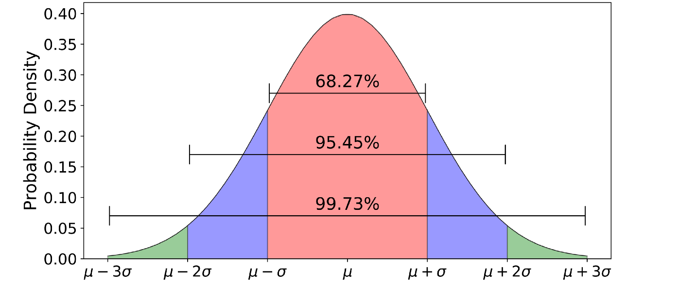
The normal (or Gaussian) distribution is the familiar “bell-shaped” curve seen in many textbooks. Its probability density is given by \(p(x) = \frac{1}{\sqrt{2\pi\sigma^2}} \exp\Big(-\frac{(x-\mu)^2}{2\sigma^2}\Big)\), where \(\mu\) is the mean and \(\sigma\) is the standard deviation.
Normal distributions occurs when there are many independent factors that combine additively, and no single one of those factors “dominates” the sum. Mathematically, this intuition is formalized through the central limit theorem.
Before continuing to read, think about examples of random variables that you expect to be normally distributed.
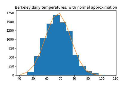
Example 1: temperature. As one example, the temperature in a given city (at a given time of year) is normally distributed, since many factors (wind, ocean currents, cloud cover, pollution) affect it, mostly independently.
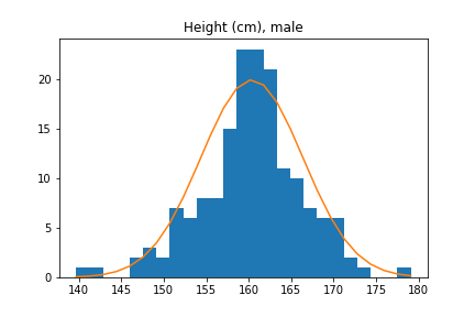
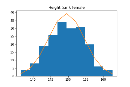
Example 2: heights. Similarly, height is normally distributed, since many different genes have some effect on height, as do other factors such as childhood nutrition.
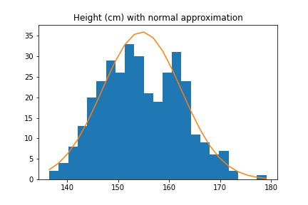
However, for height we actually have to be careful, because there are two major factors that affect height significantly: age and sex. 12-year olds are (generally) shorter than 22-year-olds, and women are on average 5 inches (13cm) shorter than men. These overlaid histograms show heights of adults conditional on sex.
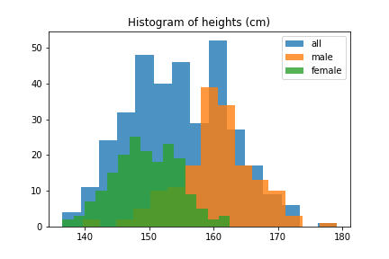
Thus, if we try to approximate the distribution of heights of all adults with a normal distribution, we will get a pretty bad approximation. However, the distribution of male heights and female heights are separately well-approximated by normal distributions.
| All | Males | Females |
|---|---|---|
 |
 |
 |
Example 3: measurement errors. Finally, the errors of a well-engineered system are often normally-distributed. One example would be a physical measurement apparatus (such as a voltmeter). Another would be the errors of a well-fit predictive model. For instance, when I was an undergraduate I fit a model to predict the pitch, yaw, roll, and other attributes of an autonomous airplane. The results are below, and all closely follow a normal distribution:

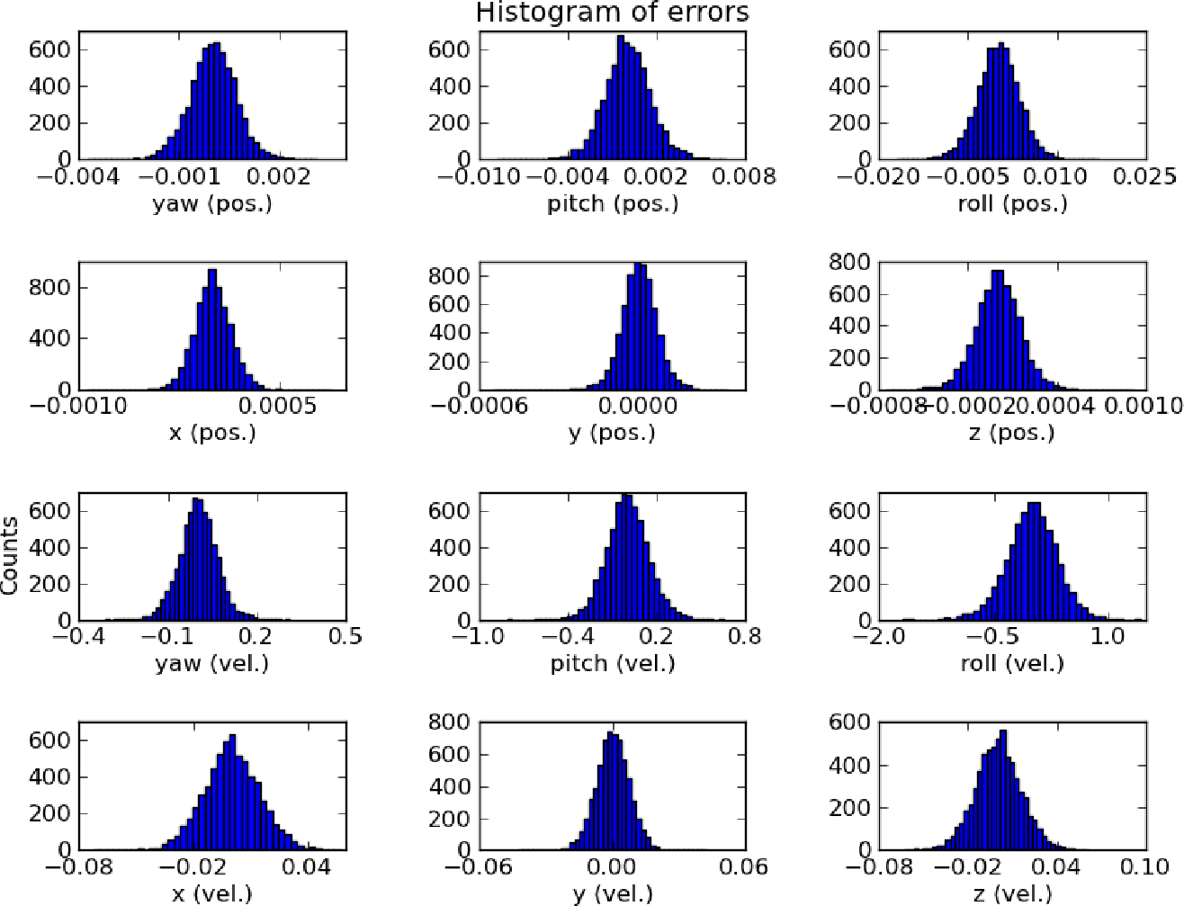
Why do well-engineered systems have normally-distributed errors? It’s a sort of reverse central limit theorem: if they didn’t, that would mean there was one large source of error that dominated the others, and a good engineer would have found and eliminated that source.
Normal distributions have thin tails (falling faster than exponential). Once we reach the extremes the tails usually underestimate the probability of rare events. As a result, we have to be careful when using a normal distribution for some of the examples above, such as heights. A normal distribution predicts that no women should be taller than 6’8”, yet there are many women who have reached this height (read more here).
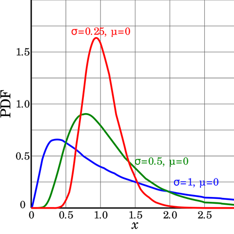
11.2 Log-normal Distributions
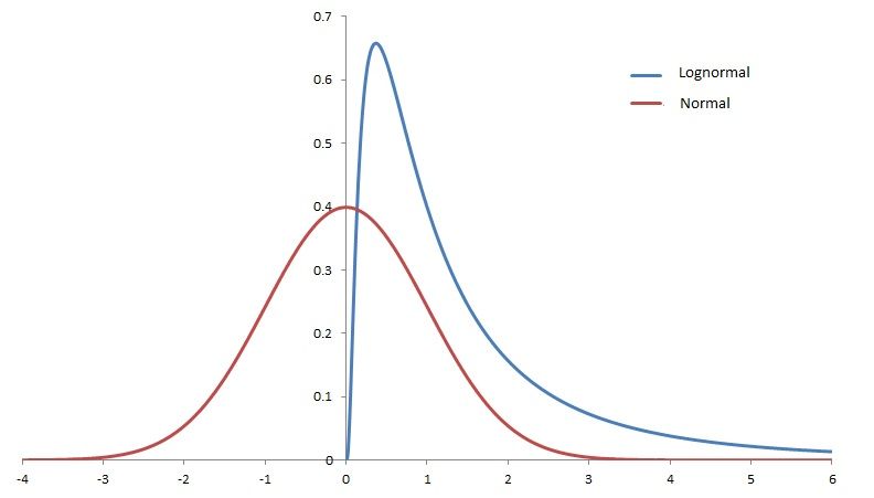
While normal distributions arise from independent additive factors, log-normal distributions arise from independent multiplicative factors (which are often more common). A random variable \(X\) is log-normally distributed if \(\log(X)\) follows a normal distribution–in other words, a log-normal distribution is what you get if you take a normal random variable and exponentiate it. Its density is given by
\(p(x) = \frac{1}{x\sqrt{2\pi\sigma^2}} \exp\Big(-\frac{(\log(x) - \mu)^2}{2\sigma^2}\Big)\).
Here \(\mu\) and \(\sigma\) are the mean and variance of \(\log(X)\) (not \(X\)).
| Examples of log-normal distributions | Log-normal(0, 1) compared to Normal(0, 1) |
|---|---|
 |
 |
Multiplicative factors tend to occur whenever there is a “growth” process over time. For instance:
- The number of employees of a company 5 years from now (or its stock price)
- US GDP in 2030
Why should we think of factors affecting a company’s employee count as multiplicative? Well, if a 20-person company does poorly it might decide to lay off 1 employee. If a 10,000-person company does poorly, it would have to lay off hundreds of employees to achieve the same relative effect. So, it makes more sense to think of “shocks” to a growth process as multiplicative rather than additive.
Log-normal distributions are much more heavy-tailed than normal distributions. One way to get a sense of this is to compare heights to stock prices.
| Height (among US adult males) | Stock price (among S&P 500 companies) | |
|---|---|---|
| Median | 175.7 cm | $119.24 |
| 99th percentile | 191.9 cm | $1870.44 |
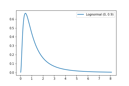
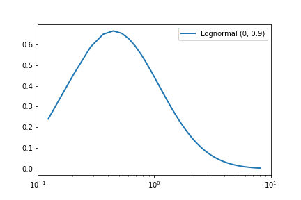
To check if a variable X is log-normal distributed, we can plot a histogram of log(X) (or equivalently, plot the x-axis on a log scale), and this should be normally distributed. For example, consider the following plots of the Lognormal(0, 0.9) distribution:
| Standard axes | Log scale x-axis |
|---|---|
 |
 |
What are other quantities that are probably log-normally distributed?
11.3 Power Law Distributions
Another common distribution is the power law distribution. Power law distributions are those that decrease at a rate of \(x\) raised to some power: \(p(x) = C / x^{\alpha}\) for some constant \(C\) and exponent \(\alpha\). (We also have to restrict \(x\) away from zero, e.g. by only considering \(x > 1\) or some other threshold.)
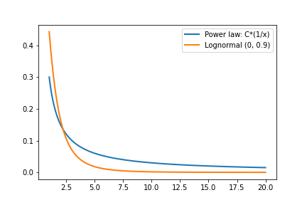
Like a log-normal distribution, power laws are heavy-tailed. In fact, they are even heavier-tailed than log-normals. To identify a power law, we can create a log-log plot (plotting both the x and y-axes on log scales). Variables that follow power laws will show a linear trend, while log-normal variables will have curvature. Here we plot the same distributions as above, but with log scale x and y axes:
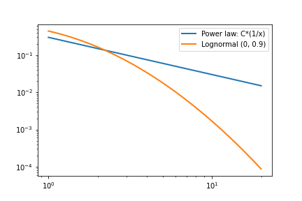
In practice, log-normal and power-law distributions often only differ far out in the tail and so it isn’t always easy (or important) to tell the difference between them.
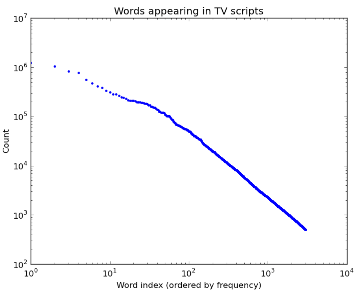
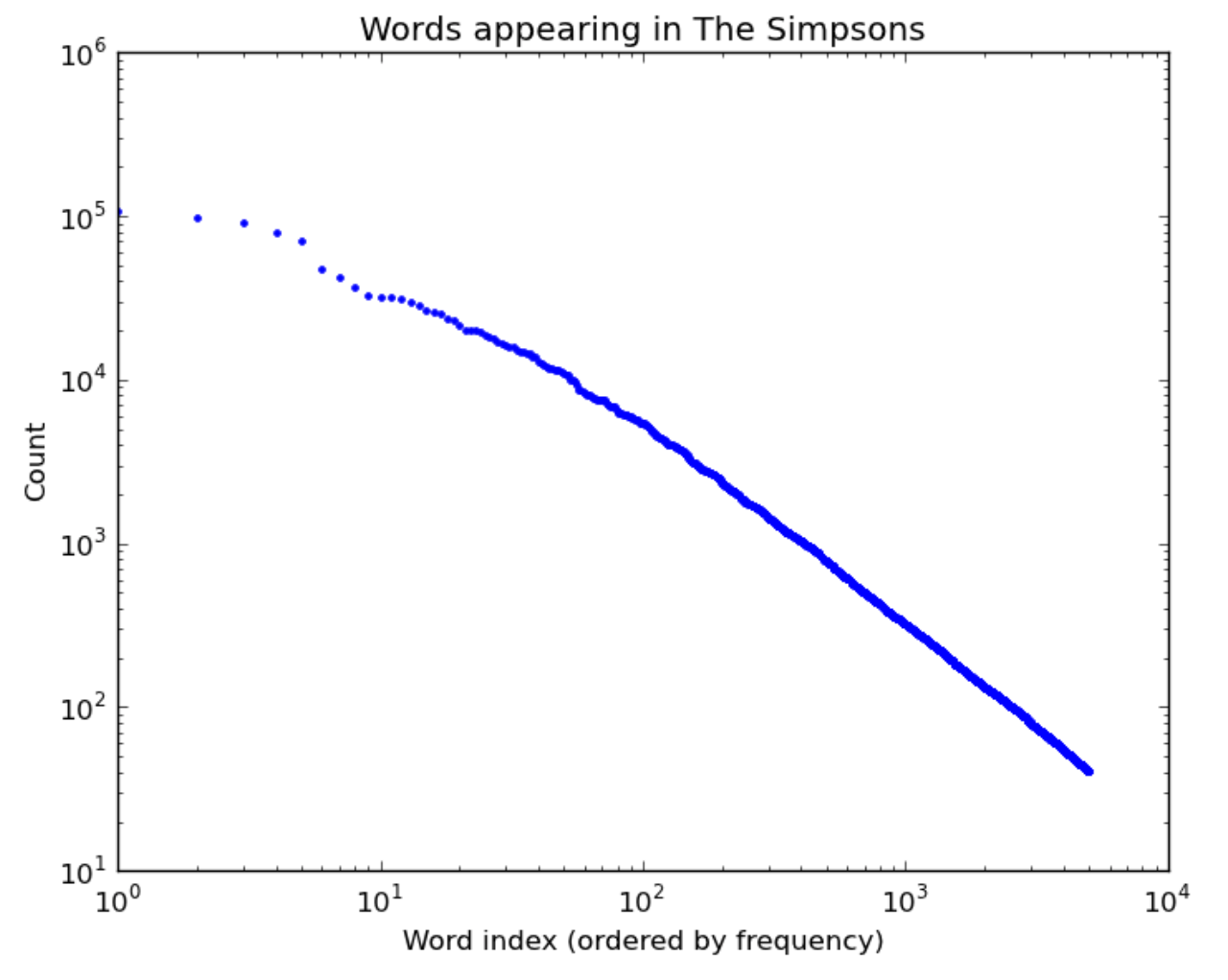
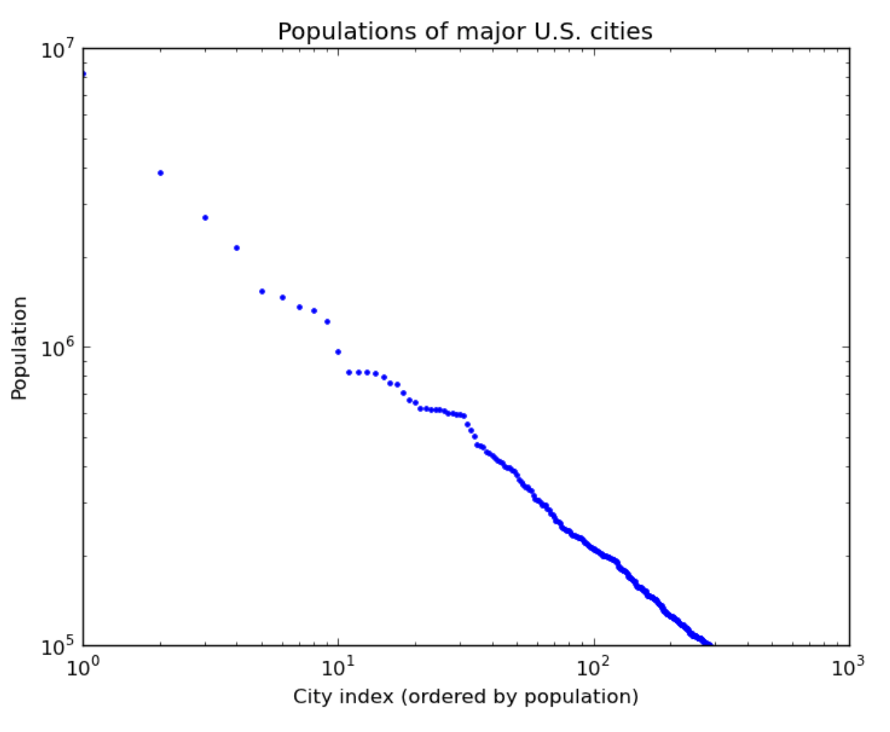
What leads to power law distributions? Here are a few real-world examples of power law distributions (plotted on a log-log scale as above):
| Words in TV scipts | Words in the Simpsons | US city populations |
|---|---|---|
 |
 |
 |
The factors that lead to power law distributions are more varied than log-normals. For a good overview, I recommend this excellent paper by Michael Mitzenmacher. I will summarize two common factors below:
One reason for power laws is that they are the unique set of scale-invariant laws: ones where \(X\) and \(2X\) (and \(3X\)) all have identical distributions. So, we should expect power laws in any case where the “units don’t matter”. Examples include the net worth of individuals (dollars are an arbitrary unit) and the size of stars (meters are an arbitrary unit, and more fundamental physical units such as the Planck length don’t generally affect stars).
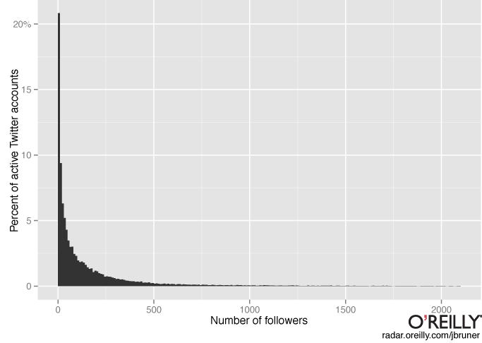
Another common reason for power laws is preferential attachment or rich get richer phenomena. An example of this would be twitter followers: once you have a lot of twitter followers, they are more likely to retweet your posts, leading to even more twitter followers. And indeed, the distribution of twitter followers is power law distributed:
“Rich get richer” also explains why words are power law distributed: the more frequent a word is, the more salient it is in most people’s minds, and hence the more it gets used in the future. And for cities, more people think of moving to Chicago (3rd largest city) than to Arlington, Texas (50th largest city) partly because Chicago is bigger.
What are other instances where we should expect to see power laws, due to either scale invariance or rich get richer?
Interestingly, in contrast to cities, country populations do not seem to fit a power law (although they could fit a mixture of two power laws reasonably):
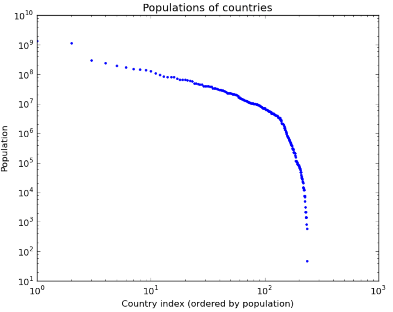
Can you think of reasons that explain this?
There is much more to be said about power laws. In addition to the Mitzenmacher paper mentioned above, I recommend this blog post by Terry Tao.
11.4 Poisson Distributions
The Poisson distribution is a discrete distribution over \(0, 1, \ldots\) (i.e. the nonnegative integers). Given a Poisson random variable \(X\) with rate \(\lambda\), the probability mass function is \(\mathbb{P}[X = k] = \frac{\lambda^k e^{-\lambda}}{k!}\).
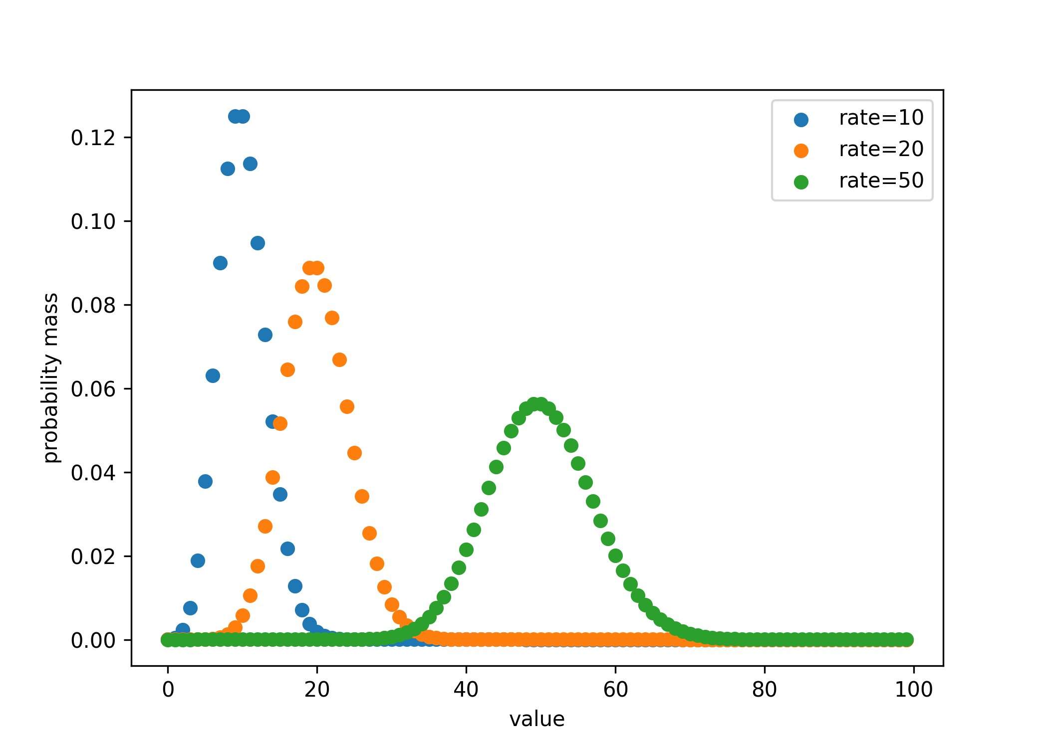
There are several notable differences between the Poisson distribution and the Gaussian distribution. First, the Poisson distribution is supported on the nonnegative integers, rather than all of \(\mathbb{R}\). Second, the tails of the Poisson distribution can be thicker than Gaussian tails. Lastly, the Poisson distribution only has one parameter, rather than two parameters, and the mean is always equal to the variance.
These properties turn out to make Poisson distributions particularly suited to capture the number of occurrences of a rare event. As a motivating example, consider the forecasting question from a past homework:
How many NYT headlines/ledes in the technology section dated between Feb 15 and Feb 21 (included) will include the terms “chatbot” or “ChatGPT”?
At each time interval (e.g. hour), we might believe that there is some small probability \(p\) that such an article will be published. When we sum over the 168 hours in a week, the expected number of articles published is \(\lambda = 168 p\), which is nonnegligible. But what is the distribution over the number of articles published? In the limit, as we make the length of the time interval go to \(0\) and scale \(p\) accordingly, the mean remains \(\lambda\) and the distribution turns out to approach a Poisson distribution with rate \(\lambda\).1
We can estimate the rate \(\lambda\) from historical data (e.g. how many news articles were published in the last 10 weeks) by leveraging the structure of Poisson distributions. In particular, a sum of Poisson distributions is itself a Poisson distribution: that is, if \(X_1\) and \(X_2\) are Poisson random variables with rates \(\lambda_1\) and \(\lambda_2\) respectively, then \(X_1 + X_2\) is a Poisson random variable with rate \(\lambda_1 + \lambda_2\). So if the news articles in one week follow a Poisson distribution with rate \(\lambda\), then the news articles across 10 weeks follow a Poisson distribution with rate \(10 \lambda\). If we have an estimate of \(10 \lambda\) from historical data across the past 10 weeks, we can divide by 10 and obtain an estimate of \(\lambda\).
We’ve gone through a lot of different distributions, and the best way to decide which distribution to use in a given forecast is through practice. Let’s conclude with an exercise that will help you practice determining which distribution to use in different contexts.
Here are a couple examples of data you might want to model. For each, would you expect its distribution to be normal, log-normal, power law, or Poisson?
- Incomes of US adults
- Citations of papers
- Number of Christmas trees sold each year
This follows from how the Poisson distribution is a limit of Binomial random variables, where the number of successes is held constant but the number of trials goes to \(\infty\).↩︎