16 Beliefs Across Time
In this lecture, we will think of beliefs as probabilities, and we will show that well-calibrated beliefs must obey certain mathematical rules across time. This can be useful in two ways:
- It allows us to assess our own calibration even before observing the outcomes of our predictions
- It makes it possible to evaluate prediction platforms, e.g. to tell whether Metaculus is behaving irrationally
As a preview, consider the following evolution over time of the probabilility assigned to an event:
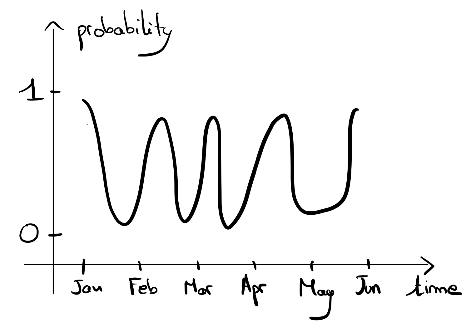
We can tell that this evolution is not good:
- Intuitively, the probability oscillates too much, which suggests that the forecaster is at times overconfident and at times underconfident.
- A bookie could easily pump money out of the forecaster if they knew in advance that the market would oscillate, by buying equal odds contracts at low price when the probability is low, and selling these contracts at a high price when the probability is high.
16.1 An example: will it rain on Friday?
Every week, on Monday and Tuesday, you are asked to predict whether it will rain on this week’s Friday. We will see how certain series of predictions cannot be well-calibrated for any possible outcome.
16.1.1 Example 1: 100% and 0%
Suppose every week, your probabilities are 100% every Monday, and 0% every Tuesday.
| Monday | Tuesday | … | Friday |
|---|---|---|---|
| 100% | 0% | … |
With these beliefs, can you be well-calibrated?
(whitespace to avoid spoilers)
…
…
…
…
…
…
…
…
…
…
…
Suppose it rains on a fraction \(\pi\) of all weeks.
| Monday | Tuesday | … | Friday |
|---|---|---|---|
| 100% | 0% | … | \(\pi\) |
Then, for your Monday predictions to be well-calibrated, you need to have \(\pi = 1\), but for your Tuesday predictions to be well-calibrated, you need to have \(\pi = 0\). This is impossible, therefore these predictions cannot be well-calibrated for any possible outcome.
16.1.2 Example 2: 80% and 20%
Suppose instead that every week, your probabilities are 80% every Monday, and 20% every Tuesday.
| Monday | Tuesday | … | Friday |
|---|---|---|---|
| 80% | 20% | … |
With these beliefs, can you be well-calibrated?
(whitespace to avoid spoilers)
…
…
…
…
…
…
…
…
…
…
…
Once again, suppose it rains on a fraction \(\pi\) of all weeks.
| Monday | Tuesday | … | Friday |
|---|---|---|---|
| 80% | 20% | … | \(\pi\) |
Then, the same reasoning shows that these predictions cannot be well-calibrated. Indeed, for your Monday predictions to be well-calibrated, you would need to have \(\pi = 0.8\), but for your Tuesday predictions to be well-calibrated, you would need to have \(\pi = 0.2\). This is impossible, therefore these predictions cannot be well-calibrated for any possible outcome.
These two examples showed that some changes in beliefs over time cannot occur if you are well-calibrated. One property these examples have in common is that your probability consistently decreases from Monday to Tuesday. After a few weeks, a better-calibrated forecaster would notice this pattern, and adjust their Monday probability accordingly.
16.1.3 Example 3: two kinds of weeks
Now, suppose that there are two kinds of weeks:
- on half of the weeks, you forecast 50% on Mondays and 60% on Tuesdays
- on the other half of the weeks, you forecast 50% on Mondays and 40% on Tuesdays
| Monday | Tuesday | … | Friday | |
|---|---|---|---|---|
| 1/2 of weeks | 50% | 60% | … | |
| 1/2 of weeks | 50% | 40% | … |
For a concrete example, suppose that after predicting on Mondays, you watch a weather forecast on TV. On half of the weeks, the TV’s forecast says that it will rain on Fridays, in which case you increase your probability to 60% on Tuesday. On the other weeks, you lower your probability to 40% on Tuesday.
With these beliefs, can you be well-calibrated?
(whitespace to avoid spoilers)
…
…
…
…
…
…
…
…
…
…
…
Suppose it rains on a fraction \(\pi_1\) of Fridays for weeks in which the TV forecast predicts rain, and a fraction \(\pi_2\) of Fridays when the TV forecast predicts no rain.
| Monday | Tuesday | … | Friday | |
|---|---|---|---|---|
| 1/2 of weeks | 50% | 60% | … | \(\pi_1\) |
| 1/2 of weeks | 50% | 40% | … | \(\pi_2\) |
Then, if \(\pi_1 = 0.6\) and \(\pi_2 = 0.4\), these predictions are well-calibrated. Indeed, in that case:
- \(p(\text{rain on Friday} \mid \text{you predicted 60\%}) = \pi_1 = 0.6\)
- \(p(\text{rain on Friday} \mid \text{you predicted 40\%}) = \pi_2 = 0.4\)
- \(p(\text{rain on Friday} \mid \text{you predicted 50\%}) = \frac 1 2 \pi_1 + \frac 1 2 \pi_2 = 0.5\)
Notice that this would not work if you had predicted 55% instead of 50% on Mondays. If that was the case, then \(p(\text{rain on Friday} \mid \text{you predicted 55\%}) = \frac 1 2 \pi_1 + \frac 1 2 \pi_2 = 0.5 \neq 55\%\).
16.2 Well-calibrated beliefs must be a Martingale
We will now describe the key property that Example 3 verified, but that Examples 1 and 2 did not: well-calibrated beliefs must be a Martingale.
Let \(p_1, ..., p_t, ...\) be the probabilities you assign to an event at different points in time. For example, in the past example, \(p_1\) would be your Monday probability of rain on Friday, and \(p_2\) would be your Tuesday probability of rain on Friday.
Qualitatively, we say that the sequence of random variables \((p_t)\) is a Martingale when the \(p_t\) stay the same in expectation. Formally, for every time step \(t \in \mathbb{N}\),
\[ \mathbb{E}[p_{t+1} \mid p_1, ..., p_t] = p_t. \]
For some extra intuition, suppose you are at time step \(t\): up to now, you have made predictions \(p_1, ..., p_t\). Between time steps \(t\) and \(t+1\), you will observe some extra information that will allow you to adjust your probability to \(p_{t+1}\). If you thought that on average this extra information would lead to a higher value of \(p_{t+1}\), i.e. \(\mathbb{E}[p_{t+1} \mid p_1, ..., p_t] > p_t\), then you should already have set \(p_t\) to this higher value!
Because well-calibrated beliefs must be a Martingale, if you find a sequence of probabilities that violates the Martingale property, you can tell that these probabilities are uncalibrated. This is useful to decide how much to trust the probabilities of forecasting platforms such as Metaculus before a question has even resolved.
Even though the Martingale property allows you to notice that something is wrong with a sequence of beliefs, it does not tell you what to do to fix it. Sometimes the beliefs alternate between extreme overconfidence and extreme underconfidence, in which case moderating the probabilities can be useful, but that is not always the only underlying issue.
16.3 Properties of Martingales
In this section, we will describe some properties of Martingales, that will make it easier for you to notice that a sequence of probabilities likely violates the Martingale property.
For example, in the motivating example at the beginning of these notes, we observed probabilities that oscillated a lot between very high and very low values. The following theorems will make precise the idea that Martingales, and therefore sequences of well-calibrated beliefs, “cannot oscillate too much”.
Our first theorem, which we present without proof, upper bounds the expected amount of variation between consecutive probabilities:
Theorem 1: Suppose \(p_1, p_2, ..., p_t, ... \in [0,1]\) is martingale. Then:
\[ \mathbb{E}\left[ \sum\limits_{t=1}^{\infty} (p_{t+1} - p_t)^2 \right] \leq p_1 (1 - p_1) \leq \frac 1 4 \]
In particular, applying Markov’s inequality allows us to upper bound the probability of large summed squared differences: for every \(x > 0\),
\[ \mathbb{P}\left[ \sum\limits_{t=1}^{\infty} (p_{t+1} - p_t)^2 \geq \frac x 4 \right] \leq \frac 1 x \]
However, a low sum of squared deviation does not preclude large oscillations. Therefore, we introduce the notion of a crossing.
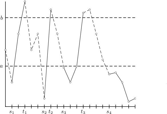
Definition: Let \(p_1, p_2, ..., p_t, ... \in [0,1]\) be a sequence of probabilities, and \(0 < a < b < 1\). We call a pair of time steps \(s < t\) a crossing if \(p_s \leq a\) and \(p_t \geq b\), or \(p_t \leq a\) and \(p_s \geq b\).
For example, in the image below, \((s_1, t_1)\), \((s_2, t_2)\), and \((s_3, t_3)\) are examples of crossings.
Our second theorem formalizes the intuition that a martingale can’t have too many crossings.
Theorem 2 (Doob’s upcrossing lemma): Suppose \(p_1, p_2, ..., p_t, ... \in [0,1]\) is martingale. Let \(K\) be the number of crossings of \((p_t)_{t\geq 1}\). Then for every \(n \geq 1\),
\[\mathbb{P}\left[ K \geq n \right] \leq \max\left(\frac a b, \frac {1-b} {1-a}\right)^n.\]
For example, if \(a = 0.2\) and \(b = 0.8\), then \(\frac a b = \frac {1-b} {1-a} = \frac 1 4\). Therefore, the probability of having 10 or more crossings is at most \(\left(\frac 1 4\right)^{10}\), which is less than one in a million.
Proof: tbd.
16.4 Conclusion
In this lecture, we saw how well calibrated beliefs must verify certain conditions across time. In particular:
- Well-calibrated beliefs are martingales, which means that they stay the same in expectation.
- Because of Doob’s upcrossing lemma, well-calibrated beliefs cannot oscillate too much between extreme values.
- Therefore, if you notice a lot of oscillations over time in your probability or the market price of a prediction market, this suggests that these predictions are uncalibrated. This can be useful to spot potential errors in forecasts before a question has resolved.