Often there are multiple ways to forecast the same thing, and we’d like a way of combining the forecasts together.
For instance, consider the following question:
How many 8.5 x 11 sheets of paper does the average tree produce?
Tip
Before continuing to read, think through how you would answer this question. Also, ask your other classmates what they would predict.
You’ll likely see that you and your classmates don’t create the same forecast for this question. This could be because you used different approaches (e.g. different reference classes) or because you had different estimates of intermediate quantities (e.g. “how many feet tall is an average tree?”). These differences suggest you might be able to improve your forecast if you and your classmates combine perspectives.
Tip
Before continuing to read, think about how you might combine multiple forecasts to create a single forecast.
In the next two lectures, we’ll discuss approaches to combine forecasts. This lecture will focus on combining point estimates and give an overview of implications for your own forecasting. Next lecture will consider more advanced methods to combine forecasts, including combining confidence intervals.
9.1 Approaches to combine point estimates
Suppose that each forecaster creates a point estimate (i.e. a single answer if the question asks for a numerical answer, or a single distribution if the question asks for a probability distribution over multiple outcomes). We consider four different approaches for combining point estimates:
Mean
Median
Trimmed mean
Weighted mean
9.1.1 Mean
The mean takes the average of the forecasts: this is the average of the answers in the case of numerical answers, and the average of the distributions in the case of probability distributions.
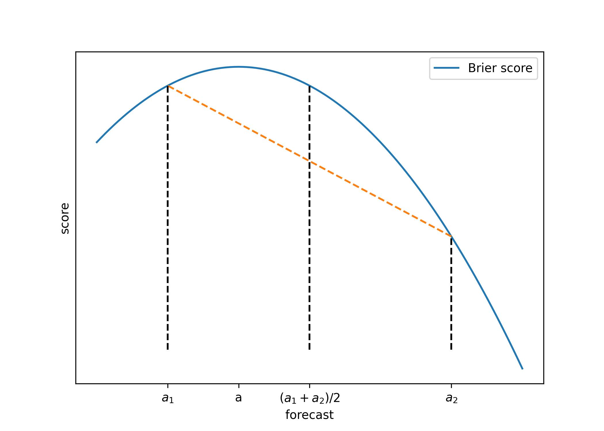
To get some intuition for why the mean performs well, let’s look at the performance of the mean under Brier’s quadratic scoring rule. Consider two forecasters who report answers of \(a_1\) and \(a_2\), respectively, and let the true answer be \(a\). The score of the average forecast \((a_1 + a_2)/2\) beats the average score of the two forecasts, as we illustrate below.
On the plot, the midpoint of the dotted orange line corresponds to \(\frac{-(a_1 - a)^2 -(a_2 - a)^2}{2}\), which is the expected score from guessing \(a_1\) or \(a_2\) with equal probability. The point on the blue curve with \(x\)-coordinate \((a_1 + a_2)/2\) corresponds to \(-(\frac{a_1 + a_2}{2} - a)^2\), which is the score of the average of the forecasts. Observe that the score \(-(\frac{a_1 + a_2}{2} - a)^2\) beats the score \(\frac{-(a_1 - a)^2 -(a_2 - a)^2}{2}\).
This observation actually generalizes to any concave scoring rule (including the log score). To formally show this, we use Jensen’s inequality, which tells us that if \(f(\cdot, \cdot)\) is a concave scoring rule, then
\(f(\frac{a_1 + a_2}{2}, a) \geq \frac{f(a_1, a) + f(a_2, a)}{2}\),
so the average forecast beats the average score of the forecasts. In fact, Jensen’s inequality tells us that if we combine \(N\) forecasts, then the average of the \(N\) forecasts similarly beats the average score of the \(N\) forecasts.
One issue with the mean is that it can swing a lot with outliers. For example, if one forecaster is way off, this significantly impacts the mean. The next two approaches avoid this issue by being robust to outliers (i.e. no single forecaster, or small group of forecasters, can affect the combined forecast too much).
9.1.2 Median
Motivated by this outlier issue, we consider the median. Unlike the mean, the median is robust to outliers. It is also independent of scale, meaning that it is the same both on the linear scale and on the log scale.
However, one disadvantage of the median is that it only considers the “middle” values, so it uses data less efficiently.
9.1.3 Trimmed Mean
Another approach that is robust to outliers is the trimmed mean. The idea is to throw out the outliers and then take the mean of the remaining forecasts. We show two ways that the trimmed mean could be instantiated.
Code
import numpy as np# Remove the top and bottom (x/2)% of data, then take mean of the remainder. def trimmed_mean_symmetric(forecasts, x): num_trim =int(forecasts.shape[0] * ((x/2.0)/100.0)) forecasts.sort() new_vals = forecasts[num_trim:forecasts.shape[0]-num_trim]return np.mean(new_vals)# Remove the x% of data that is furthest from mean, then take the mean of the remainder. def trimmed_mean_distance(forecasts, x): mean_val = np.mean(forecasts) num_trim =int(forecasts.shape[0] * (x/100.0)) dist_from_mean = np.abs(forecasts - mean_val) indices = dist_from_mean.argsort() new_vals = forecasts[indices[:-num_trim]]return np.mean(new_vals)
The trimmed mean keeps some of the desirable properties of both the mean and the median. Like the median, it is robust to outliers. Like the mean, it makes use of (most of) the distribution of forecasts rather than just the middle forecast.
Interestingly, for probabilities, the trimmed mean implicitly “extremizes” the forecast, as we show in an example below:
Code
# Probability forecasts of 100 students forecasts = np.zeros(100) for i inrange(100):if i <95: # 95 people give p = 0.99 forecasts[i] =0.99else: # 5 people give p = 0.5 forecasts[i] =0.5mean_value = np.mean(forecasts)trimmed_mean_symmetric_value = trimmed_mean_symmetric(forecasts, 10)trimmed_mean_distance_value = trimmed_mean_distance(forecasts, 10)print("mean: "+str(np.mean(forecasts)))print(f'trimmed mean (version 1): {trimmed_mean_symmetric_value}')print(f'trimmed mean (version 2): {trimmed_mean_distance_value}')
mean: 0.9654999999999998
trimmed mean (version 1): 0.99
trimmed mean (version 2): 0.99
In this example, the trimmed mean makes the probability closer to \(1\) than the mean.
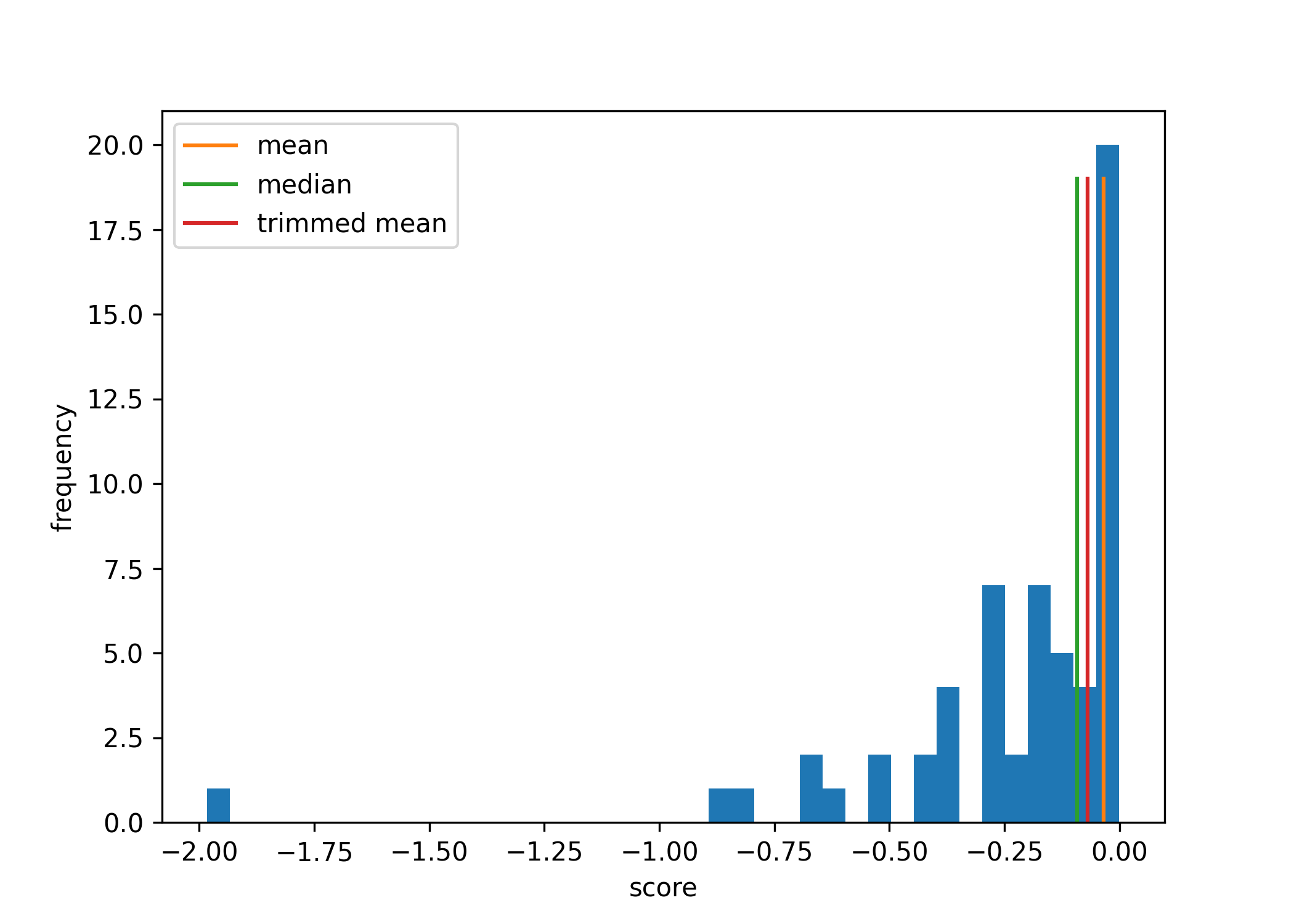
Comparison of these approaches. As an illustration of these 3 approaches—the mean, the median, and the trimmed mean—let’s consider a dataset of forecasts (the forecasts in the Spring 2022 offering of this class).
We first consider the performance of the 3 combined forecasts on a single question, relative to the performance of students in the class.
On this question, the mean outperforms 67.8% of students, the median outperforms 61.0% of students, and the trimmed mean outperforms 62.7% of students.
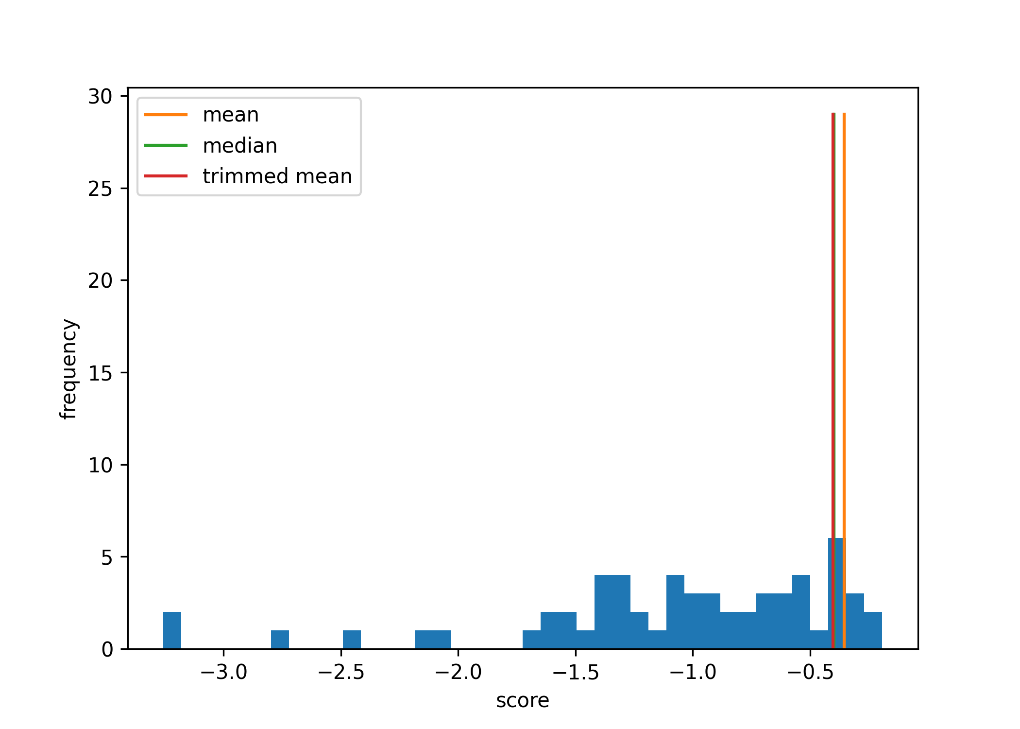
The performance of these combined forecasts is amplified when we consider aggregate performance across several questions. To show this, we consider the overall performance across 5 questions in the dataset.
The mean outperforms 91.5% of students, the median outperforms 68.4% of students, and the trimmed mean outperforms 86.4% of students.
9.1.4 Weighted Mean
We might not want to treat different forecasters equally. For example, we might not want to place the same weight on the prediction of a beginning forecaster as the prediction of an expert forecaster. Or, if a forecaster tells us that they are not confident about their prediction, we might want to lower how much we consider their forecast.
The weighted mean is a generalization of the mean that allows us to place different weights on different forecasters. The idea is to assign each forecaster a weight and then take the weighted average of the forecasts. These weights could be set by looking at the historical performance of forecasters or by explicitly asking forecasts about their confidence level.
The weighted mean has two interesting connections to the mean and the trimmed mean. First, like the mean, by Jensen’s inequality, for any concave scoring rule, the weighted mean outperforms the weighted average of the forecasts. Second, the trimmed mean is actually a special case of the weighted mean that sets the weights of outliers to 0.
9.2 Implications for your own forecasting
Now that we’ve described a bunch of approaches to combine forecasts, let’s look at how you could use these ideas to actually improve your own predictions. We provide three concrete approaches, each of which we’ll explore in more depth in the next lecture.
Weight experts: When deciding what to believe, weigh various sources by how much you trust them and take a weighted average.
Work with other people: Forecast in teams and combine the forecasts of different team members. (Related to this is the Delphi method, which we’ll discuss next time.)
Ensemble with yourself: Think of a number a few different times and take the average. For example, I often waffle back and forth on what number to go with; sometimes it’s best to just take the average of numbers you’ve considered and call it a day.